Category Archives: Graph ur world
Wakanda (Black Panther) Geography Now!”
Top Google Searches Coming From Syria
Pareto principle
From Wikipedia, the free encyclopedia
For the optimal allocation of resources, see Pareto efficiency.
The Pareto principle (also known as the 80–20 rule, the law of the vital few, and the principle of factor sparsity) states that, for many events, roughly 80% of the effects come from 20% of the causes.[1]Management consultantJoseph M. Juran suggested the principle and named it after Italian economistVilfredo Pareto, who, while at theUniversity of Lausanne in 1896, published his first paper “Cours d’économie politique.” Essentially, Pareto showed that approximately 80% of the land in Italy was owned by 20% of the population; Pareto developed the principle by observing that 20% of the peapods in his garden contained 80% of the peas.[citation needed]
It is a common rule of thumb in business; e.g., “80% of your sales come from 20% of your clients.” With respect to this article, 80% of the value will come from 20% of the content. Mathematically, the 80–20 rule is roughly followed by a power law distribution (also known as a Pareto distribution) for a particular set of parameters, and many natural phenomena have been shown empirically to exhibit such a distribution.[2]
The Pareto principle is only tangentially related to Pareto efficiency. Pareto developed both concepts in the context of the distribution of income and wealth among the population.
In economics[edit]
The original observation was in connection with population and wealth. Pareto noticed that 80% of Italy’s land was owned by 20% of the population.[3] He then carried out surveys on a variety of other countries and found to his surprise that a similar distribution applied.
A chart that gave the inequality a very visible and comprehensible form, the so-called ‘champagne glass’ effect,[4] was contained in the 1992 United Nations Development Program Report, which showed the distribution of global income to be very uneven, with the richest 20% of the world’s population controlling 82.7% of the world’s income.[5]
| Quintile of population | Income |
|---|---|
| Richest 20% | 82.70% |
| Second 20% | 11.75% |
| Third 20% | 2.30% |
| Fourth 20% | 1.85% |
| Poorest 20% | 1.40% |
In business[edit]
80% of a company’s profits come from 20% of its customersThe distribution is claimed to appear in several different aspects relevant to entrepreneurs and business managers. For example:
- 80% of a company’s complaints come from 20% of its customers
- 80% of a company’s profits come from 20% of the time its staff spend
- 80% of a company’s sales come from 20% of its products
- 80% of a company’s sales are made by 20% of its sales staff[7]
Therefore, many businesses have an easy access to dramatic improvements in profitability by focusing on the most effective areas and eliminating, ignoring, automating, delegating or retraining the rest, as appropriate.[citation needed]
Limited applicability to science[edit]
|
|
This article is written like a research paper or scientific journal that may use overly technical terms or may not be written like an encyclopedic article. (June 2015) |
The more unified a theory is, the more predictions it makes, and the greater the chance is of some of them being cheaply testable. Modifications of existing theories makes much fewer new and unique predictions, increasing the risk of the few there is all being very expensive to test.[8] If the Pareto principle or any other kind of increased costs were the cause of stagnation in the unification of especially physics, the modification of existing theories would have been even more severely slowed down than ever the unification by breakthroughs.[9][10]
In software[edit]
In computer science and engineering control theory, such as for electromechanical energy converters, the Pareto principle can be applied to optimization efforts.[11]
For example, Microsoft noted that by fixing the top 20% of the most-reported bugs, 80% of the related errors and crashes in a given system would be eliminated.[12]
In load testing, it is common practice to estimate that 80% of the traffic occurs during 20% of the time.[citation needed]
In software engineering, Lowell Arthur expressed a corollary principle: “20 percent of the code has 80 percent of the errors. Find them, fix them!”[13]
Occupational health and safety[edit]
The Pareto principle is used in occupational health and safety to underline the importance of hazard prioritization. Assuming 20% of the hazards will account for 80% of the injuries and by categorizing hazards, safety professionals can target those 20% of the hazards that cause 80% of the injuries or accidents. Alternatively, if hazards are addressed in random order, then a safety professional is more likely to fix one of the 80% of hazards which account for some fraction of the remaining 20% of injuries.[14]
Aside from ensuring efficient accident prevention practices, the Pareto principle also ensures hazards are addressed in an economical order as the technique ensures the resources used are best used to prevent the most accidents.[15]
Other applications[edit]
In the systems science discipline, Epstein and Axtell created an agent-based simulation model called SugarScape, from a decentralized modeling approach, based on individual behavior rules defined for each agent in the economy. Wealth distribution and Pareto’s 80/20 principle became emergent in their results, which suggests the principle is a natural phenomenon.[16]
The Pareto principle has many applications in quality control.[citation needed] It is the basis for the Pareto chart, one of the key tools used in total quality control and six sigma. The Pareto principle serves as a baseline for ABC-analysis and XYZ-analysis, widely used in logistics and procurement for the purpose of optimizing stock of goods, as well as costs of keeping and replenishing that stock.[17]
The Pareto principle was also mentioned in the book 24/8 – The Secret for being Mega-Effective by Achieving More in Less Time by Amit Offir. Offir claims that if you want to function as a one-stop shop, simply focus on the 20% of what is important in a project and that way you will save a lot of time and energy.
In health care in the United States, 20% of patients have been found to use 80% of health care resources.[18]
Several criminology studies have found 80% of crimes are committed by 20% of criminals.[citation needed]This statistic is used to support both stop-and-frisk policies and broken windows policing, as catching those criminals committing minor crimes will likely net many criminals wanted for (or who would normally commit) larger ones.
In the financial services industry, this concept is known as profit risk, where 20% or fewer of a company’s customers are generating positive income, while 80% or more are costing the company money.[19]
Mathematical notes[edit]
The idea has rule of thumb application in many places, but it is commonly misused. For example, it is a misuse to state a solution to a problem “fits the 80–20 rule” just because it fits 80% of the cases; it must also be that the solution requires only 20% of the resources that would be needed to solve all cases. Additionally, it is a misuse of the 80–20 rule to interpret data with a small number of categories or observations.
This is a special case of the wider phenomenon of Pareto distributions. If the Pareto indexα, which is one of the parameters characterizing a Pareto distribution, is chosen asα = log45 ≈ 1.16, then one has 80% of effects coming from 20% of causes.
It follows that one also has 80% of that top 80% of effects coming from 20% of that top 20% of causes, and so on. Eighty percent of 80% is 64%; 20% of 20% is 4%, so this implies a “64-4” law; and similarly implies a “51.2-0.8” law. Similarly for the bottom 80% of causes and bottom 20% of effects, the bottom 80% of the bottom 80% only cause 20% of the remaining 20%. This is broadly in line with the world population/wealth table above, where the bottom 60% of the people own 5.5% of the wealth.
The 64-4 correlation also implies a 32% ‘fair’ area between the 4% and 64%, where the lower 80% of the top 20% (16%) and upper 20% of the bottom 80% (also 16%) relates to the corresponding lower top and upper bottom of effects (32%). This is also broadly in line with the world population table above, where the second 20% control 12% of the wealth, and the bottom of the top 20% (presumably) control 16% of the wealth.
The term 80–20 is only a shorthand for the general principle at work. In individual cases, the distribution could just as well be, say, 80–10 or 80–30. There is no need for the two numbers to add up to the number 100, as they are measures of different things, e.g., ‘number of customers’ vs ‘amount spent’). However, each case in which they do not add up to 100%, is equivalent to one in which they do; for example, as noted above, the “64-4 law” (in which the two numbers do not add up to 100%) is equivalent to the “80–20 law” (in which they do add up to 100%). Thus, specifying two percentages independently does not lead to a broader class of distributions than what one gets by specifying the larger one and letting the smaller one be its complement relative to 100%. Thus, there is only one degree of freedom in the choice of that parameter.
Adding up to 100 leads to a nice symmetry. For example, if 80% of effects come from the top 20% of sources, then the remaining 20% of effects come from the lower 80% of sources. This is called the “joint ratio”, and can be used to measure the degree of imbalance: a joint ratio of 96:4 is very imbalanced, 80:20 is significantly imbalanced (Gini index: 60%), 70:30 is moderately imbalanced (Gini index: 40%), and 55:45 is just slightly imbalanced.
The Pareto principle is an illustration of a “power law” relationship, which also occurs in phenomena such as brush fires and earthquakes.[20] Because it is self-similar over a wide range of magnitudes, it produces outcomes completely different from Gaussian distribution phenomena. This fact explains the frequent breakdowns of sophisticated financial instruments, which are modeled on the assumption that a Gaussian relationship is appropriate to, for example, stock price movements.[21]
Equality measures[edit]
Gini coefficient and Hoover index[edit]
Using the “A : B” notation (for example, 0.8:0.2) and with A + B = 1, inequality measures like the Gini index (G) and the Hoover index (H) can be computed. In this case both are the same.


Theil index[edit]
The Theil index is an entropy measure used to quantify inequalities. The measure is 0 for 50:50 distributions and reaches 1 at a Pareto distribution of 82:18. Higher inequalities yield Theil indices above 1.[22]

See also
The Zipf Mystery
From Wikipedia, the free encyclopedia
|
Probability mass function
|
|
|
Cumulative distribution function
|
|
| Parameters |  (real) (real) (integer) (integer) |
|---|---|
| Support |  |
| pmf |  |
| CDF |  |
| Mean |  |
| Mode |  |
| Entropy |  |
| MGF |  |
| CF |  |


Zipf’s law /ˈzɪf/, an empirical law formulated using mathematical statistics, refers to the fact that many types of data studied in the physical and social sciences can be approximated with a Zipfian distribution, one of a family of related discrete power law probability distributions. The law is named after the American linguist George Kingsley Zipf (1902–1950), who popularized it and sought to explain it (Zipf 1935, 1949), though he did not claim to have originated it.[1] The French stenographer Jean-Baptiste Estoup (1868–1950) appears to have noticed the regularity before Zipf.[2] It was also noted in 1913 by German physicist Felix Auerbach[3] (1856–1933).
Motivation[edit]
Zipf’s law states that given some corpus of natural language utterances, the frequency of any word is inversely proportionalto its rank in the frequency table. Thus the most frequent word will occur approximately twice as often as the second most frequent word, three times as often as the third most frequent word, etc. For example, in the Brown Corpus of American English text, the word “the” is the most frequently occurring word, and by itself accounts for nearly 7% of all word occurrences (69,971 out of slightly over 1 million). True to Zipf’s Law, the second-place word “of” accounts for slightly over 3.5% of words (36,411 occurrences), followed by “and” (28,852). Only 135 vocabulary items are needed to account for half the Brown Corpus.[4]
The same relationship occurs in many other rankings unrelated to language, such as the population ranks of cities in various countries, corporation sizes, income rankings, ranks of number of people watching the same TV channel,[5] and so on. The appearance of the distribution in rankings of cities by population was first noticed by Felix Auerbach in 1913.[3]Empirically, a data set can be tested to see whether Zipf’s law applies by checking the goodness of fit of an empirical distribution to the hypothesized power law distribution with a Kolmogorov-Smirnov test, and then comparing the (log) likelihood ratio of the power law distribution to alternative distributions like an exponential distribution or lognormal distribution.[6] When Zipf’s law is checked for cities, a better fit has been found with b = 1.07; i.e. the  largest settlement is
  the size of the largest settlement. While Zipf’s law holds for the upper tail of the distribution, the entire distribution of cities is log-normal and follows Gibrat’s law.[7] Both laws are consistent because a log-normal tail can typically not be distinguished from a Pareto (Zipf) tail.
Theoretical review[edit]
Zipf’s law is most easily observed by plotting the data on a log-log graph, with the axes being log (rank order) and log (frequency). For example, the word “the” (as described above) would appear at x = log(1), y = log(69971). It is also possible to plot reciprocal rank against frequency or reciprocal frequency or interword interval against rank.[1] The data conform to Zipf’s law to the extent that the plot is linear.
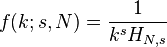
Formally, let:
- N be the number of elements;
- k be their rank;
- s be the value of the exponent characterizing the distribution.
Zipf’s law then predicts that out of a population of N elements, the frequency of elements of rank k, f(k;s,N), is:

Zipf’s law holds if the number of occurrences of each element are independent and identically distributed random variables with power law distribution 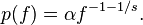 [8]
[8]
In the example of the frequency of words in the English language, N is the number of words in the English language and, if we use the classic version of Zipf’s law, the exponent sis 1. f(k; s,N) will then be the fraction of the time the kth most common word occurs.
The law may also be written:
where HN,s is the Nth generalized harmonic number.
The simplest case of Zipf’s law is a “1⁄f function”. Given a set of Zipfian distributed frequencies, sorted from most common to least common, the second most common frequency will occur ½ as often as the first. The third most common frequency will occur ⅓ as often as the first. The nth most common frequency will occur 1⁄n as often as the first. However, this cannot hold exactly, because items must occur an integer number of times; there cannot be 2.5 occurrences of a word. Nevertheless, over fairly wide ranges, and to a fairly good approximation, many natural phenomena obey Zipf’s law.
Mathematically, the sum of all relative frequencies in a Zipf distribution is equal to the harmonic series, and

In human languages, word frequencies have a very heavy-tailed distribution, and can therefore be modeled reasonably well by a Zipf distribution with an s close to 1.
As long as the exponent s exceeds 1, it is possible for such a law to hold with infinitely many words, since if s > 1 then

where ζ is Riemann’s zeta function.
Statistical explanation[edit]
It is not known why Zipf’s law holds for most languages.[9] However, it may be partially explained by the statistical analysis of randomly generated texts. Wentian Li has shown that in a document in which each character has been chosen randomly from a uniform distribution of all letters (plus a space character), the “words” follow the general trend of Zipf’s law (appearing approximately linear on log-log plot).[10] Vitold Belevitch in a paper, On the Statistical Laws of Linguistic Distribution offered a mathematical derivation. He took a large class of well-behaved statistical distributions (not only the normal distribution) and expressed them in terms of rank. He then expanded each expression into a Taylor series. In every case Belevitch obtained the remarkable result that a first-order truncation of the series resulted in Zipf’s law. Further, a second-order truncation of the Taylor series resulted in Mandelbrot’s law.[11][12]
The principle of least effort is another possible explanation: Zipf himself proposed that neither speakers nor hearers using a given language want to work any harder than necessary to reach understanding, and the process that results in approximately equal distribution of effort leads to the observed Zipf distribution.[13][14]
Related laws[edit]

A plot of word frequency in Wikipedia (November 27, 2006). The plot is in log-log coordinates. x is rank of a word in the frequency table; y is the total number of the word’s occurrences. Most popular words are “the”, “of” and “and”, as expected. Zipf’s law corresponds to the middle linear portion of the curve, roughly following the green (1/x) line, while the early part is closer to the magenta (1/”x^0.5″) line while the later part is closer to the cyan (1/”(k+x)^2.0″) line. These lines correspond to three distinct parameterizations of the Zipf-Mandelbrot distribution.
Zipf’s law in fact refers more generally to frequency distributions of “rank data,” in which the relative frequency of the nth-ranked item is given by the Zeta distribution, 1/(nsζ(s)), where the parameter s > 1 indexes the members of this family ofprobability distributions. Indeed, Zipf’s law is sometimes synonymous with “zeta distribution,” since probability distributions are sometimes called “laws”. This distribution is sometimes called the Zipfian or Yule distribution.
A generalization of Zipf’s law is the Zipf–Mandelbrot law, proposed by Benoît Mandelbrot, whose frequencies are:
![f(k;N,q,s)=\frac{[\mbox{constant}]}{(k+q)^s}.\,](https://upload.wikimedia.org/math/1/b/6/1b692df3c837478895f4e8afafa07c25.png)
The “constant” is the reciprocal of the Hurwitz zeta function evaluated at s. In practice, as easily observable in distribution plots for large corpora, the observed distribution can better be modelled as a sum of separate distributions for different subsets or subtypes of words that follow different parameterizations of the Zipf-Mandelbrot distribution, in particular the closed class of functional words exhibit “s” lower than 1, while open-ended vocabulary growth with document size and corpus size require “s” greater than 1 for convergence of the Generalized Harmonic Series.[1]
Zipfian distributions can be obtained from Pareto distributions by an exchange of variables.[15]
The Zipf distribution is sometimes called the discrete Pareto distribution[16] because it is analogous to the continuousPareto distribution in the same way that the discrete uniform distribution is analogous to the continuous uniform distribution.
The tail frequencies of the Yule–Simon distribution are approximately
![f(k;\rho) \approx \frac{[\mbox{constant}]}{k^{\rho+1}}](https://upload.wikimedia.org/math/7/6/0/760a3313829267bf212b9b153158ca80.png)
for any choice of ρ > 0.
In the parabolic fractal distribution, the logarithm of the frequency is a quadratic polynomial of the logarithm of the rank. This can markedly improve the fit over a simple power-law relationship.[15] Like fractal dimension, it is possible to calculate Zipf dimension, which is a useful parameter in the analysis of texts.[17]
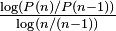
It has been argued that Benford’s law is a special bounded case of Zipf’s law,[15] with the connection between these two laws being explained by their both originating from scale invariant functional relations from statistical physics and critical phenomena.[18] The ratios of probabilities in Benford’s law are not constant. The leading digits of data satisfying Zipf’s law with s = 1 satisfies Benford’s law.
 |
Benford’s law:  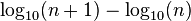 |
 |
|---|---|---|
| 1 | 0.30103000 | |
| 2 | 0.17609126 | -0.7735840 |
| 3 | 0.12493874 | -0.8463832 |
| 4 | 0.09691001 | -0.8830605 |
| 5 | 0.07918125 | -0.9054412 |
| 6 | 0.06694679 | -0.9205788 |
| 7 | 0.05799195 | -0.9315169 |
| 8 | 0.05115252 | -0.9397966 |
| 9 | 0.04575749 | -0.9462848 |
Zipf’s distribution is also applied to estimate the emergent value of networked systems and also service-oriented environments
Total Chaos: Massive Market Moves Spark Selling-Panic Into Close
Submitted by Tyler Durden
Perhaps this sums up the day for many FX, bond, equity, and oil traders today…

Incredible Volatility today – 100 point roundtrip in the S&P, and 800 points in the Dow – all driven by a halt in Ruble Trading, the European close, and Kuwait pissing on the US market’s fireworks…

Today’s melt-up into the European close was the biggst of the year…
And the volatility was incredible across the entire US equity market – as the S&P ramp ran stops to yesterday’s highs then gave it all back...again around the EU close

Close-up on S&P 500 e-minis… the machines ran all the stops everywhere today…

A massive roundtrip in cash markets…

Leaving most of the major indices down over 5% from all-time-highs…

Financials starting to show some risk…

The Russian markets dominated headlines…

but the US credit markets were more worrisome as it appears the risk has finally started to appear in the investment-grade credit market.
High yield bond yields hit 2-year highs… and spreads to 18 month wides…

And Investment Grade credit has become infected…

Longer-term…

Every asset class underwent a roller-coaster…
Treasury yields fell 10ps, rose 10bps then fell 8bps…

and the Treasury yield curve is following the exact smae trajectory as it did into the last recession/tightening..

Silver and Gold pumped and dumped.. as oil dumped and pumped and dumped…

FX markets turmoiled leasving the USD lower on the day but USDJPY wa sin charge of stocks – and major unwinds into the close – which is very unusual ahead of FOMC tomorrow and Japan tonioght

Across the asset classes today – these were the events..

Finally we wonder… who was this mysterious $3.7 billion trader today…
But don;t forget…
Charts: Bloomberg
Just What Is China Buying?
Submitted by Tyler Durden
Something strange is going on in China. On one hand, as the chart below shows, China’s trade surplus is growing and growing, and just hit record highs. In other words, China is – on paper – receiving record amounts of foreign currencies in exchange for its (mostly) goods exports.
That much is clear in the Chinese (record) trade balance chart below:

Yet on the other hand, a chart from Deutsche Bank shows something very peculiar: even as China’s foreign reserves should be rising, they are not only dropping, but just suffered their biggest quarterly drop in the past decade!

This validates what the TIC data has shown recently, namely that China has not only not been adding to US Treasury but reduced its TSY holdings to the lowest since February 2013, and that contrary to what some have alleged, China is not using Belgium as an offshore-based conduit for Treasury accumulation.

A bigger question is just what is China buying “off the books” to account for this reserve decline, amounting to about $100 billion in Q3, or is this merely due to even more off the books “capital flight” as some has speculated. Or is China indeed actively buying commodities – either as shown here previously for Commodity Funding Deals involving goldor in physical bulk, perhaps to quietly fill up its new Strategic Petroleum Reserve (see “Record Oil Tankers Sailing to China Amid Stockpiling Signs“) – and bypassing the official ledger in doing so. If so, which commodities is China buying, and how big will the foreign reserve plunge be in the fourth quarter.
For the answer to the latter we will check back in a little over a month when the “official” data is released. As for the former, one can only speculate.
Average:
Awwww…Muslim welfare leeches in Britain suffering from a housing/employment crisis, largely created by massive Muslim immigration
As they say, what goes around, comes around.


Mapping Recent “Incidents” Between Russia And NATO
by Tyler Durden
Having previously shown the dramatic build-up of NATO fighter jets around Russia‘s border, we thought mapping the rising number of “incidents” – which are worse than during the cold war – between NATO and Russia this year would be useful…

It appears Finland and Sweden are the most at risk of a major ‘incident’.
The 10 Corporations That Control Almost Everything You Buy
Submitted by Tyler Durden
We know the ten “people” that run the world, that 25 cities represent over half the world’s GDP, and that theworld’s billionaires control a stunning $33 trillion in net worth… but who controls what the average joe-sixpack on Main Street buys? As PolicyMic notes, these ten mega corporations control the output of almost everything we buy – from household products to pet food and from jeans to jello. The so-called “Illusion of Choice,” that these corporations (and their nepotistic inter-relationships) create is remarkable…
(click image for gigantic legible version)

(Note: The chart shows a mix of networks. Parent companies may own, own shares of, or may simply partner with their branch networks. For example, Coca-Cola does not own Monster, but distributes the energy drink. Another note: We are not sure how up-to-date the chart is. For example, it has not been updated to reflect P&G’s sale of Pringles to Kellogg’s in February.)
Here are just a few examples: Yum Brands owns KFC and Taco Bell. The company was a spin-off of Pepsi. All Yum Brands restaurants sell only Pepsi products because of a special partnership with the soda-maker.
$84 billion-company Proctor & Gamble — the largest advertiser in the U.S. — is paired with a number of diverse brands that produce everything from medicine to toothpaste to high-end fashion. All tallied, P&G reportedly serves a whopping 4.8 billion people around the world through this network.
$200 billion-corporation Nestle — famous for chocolate, but which is the biggest food company in the world — owns nearly 8,000 different brands worldwide, and takes stake in or is partnered with a swath of others. Included in this network is shampoo company L’Oreal, baby food giant Gerber, clothing brand Diesel, and pet food makers Purina and Friskies.
Unilever, of soap fame, reportedly serves 2 billion people around the world, controlling a network that produces everything from Q-tips to Skippy peanut butter.
